Functional Raycasting Renderer
This part describes a basic raycaster.
You can play around with the live demo at raycaster-demo or the source code at github.
The demo and the code examples are written in ClojureScript following a (mostly) functional style. However the concepts described here should be applicable to any language.
One could say that ray casting is a form of “fake” 3D, which, I guess, is why it’s sometimes called 2.5D. Some popular examples of ray casters where the 90’s first person shooters like Wolfenstein 3D, Duke Nukem 3D and the like, which used raycasting in one form or another to draw their scenes. The reason why these games can’t be called true 3D is because they are actually 2D games under the covers. For instance Wolfenstein 3D is nothing more than a simple 2D tile game. Everything in it happens on a flat grid and all of the game logic is limited to two dimensions. The only 3D part of it is the rendering of that 2D data, nothing else. Raycasting was also a neat way to get “cheap” 3D before computers got fast enough to run real 3D engines.
Basics
As you might imagine ray casting has something to do with casting rays, but to figure out exactly what, it’s useful for us to change our point of view for a moment. Imagine a 2D map filled with objects. You’re probably picturing it top down, seeing every object from above. Now imagine actually being on that map and not just looking from above, but being on that 2D plane. You wouldn’t see much, in fact you would just see a bunch of lines and wouldn’t be able to tell exactly what they represent, nor how far away a particular objects might be. Take for example this square:
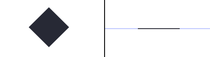
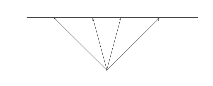
You can see that when we look at it sideways it’s hard to tell if the thing we are looking at is a square or not, or how many sides do we see, or how far away it is. There is just not enough information to tell. This is where ray casting can help us figure these things out. Ray casting lets us probe the distance between our eye and a point in the distance. We can imagine casting a ray as extending a line from our eye across a plane until it hits an obstacle. To get a good idea of that we are looking at, we cast many rays across our field of vision. The more rays we cast the more information we gather about the object in the distance.
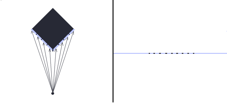
Once we have the ray lengths we can figure out the distance and the shape of the object we are looking at. You can see from the picture above that each ray represents a distance from our eye to a segment of the object. With this information we can visualize depth by drawing a vertical column for each segment of the object. We draw these columns by extending them below and above the line of the object. The actual height of these columns is determined by the length of the ray that hit the section, the longer the ray the shorter the column since it represents a more distant section of the object and vice versa.
Here’s how it would look if we had drawn the example from above to the screen:
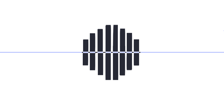
Not very realistic, but if we squint hard enough we can see something that resembles a cube! And if we wanted, we could have cast more rays to get a smoother image.
As far as the general idea goes, this is as much as there is to it!
Casting rays
Now that we have the general idea of what we are trying to do, it’s time to think about how to implement it. The first thing that we have to do is to figure out how exactly do we cast a ray across a plane. So far we have thought about casting rays as smoothly extending them from our eye until they would hit an obstacle in the distance. This is a nice way to think about it, but unfortunately this way of thinking is not very useful when we try to implement it. If we were to do it like that, we would have to check every single point along the way. And we certainly wouldn’t get very far with that approach since we would have to check an infinite number of points! Obviously we would have to extend the ray in discrete steps. However, even with this approach, there would still be some problems that we would have to address.
One of the problems with extending a ray in discrete steps is the possibility of completely missing an object
even though the object itself is in the path of the ray as shown by this animation:

You can see that the ray just keeps going, failing to detect the square that was in its path.
Another problem would be if our ray actually hit the object, but the point of contact was inside the of the
object and not on the edge.

Even though the ray actually stopped on the object and didn’t fly off into infinity, we would still get an incorrect distance to it, because it’s actually the distance to the edge what we’re trying to get.
In fact it’s very unlikely that we’d ever actually hit an edge of an object using this method. We would have to come up with something better than just extending the ray from us and hoping to randomly hit something. We would need a way to jump across the plane in discrete steps without jumping over any objects or stopping inside of them. One easy solution to this problem would be to place all object on a grid. By doing this we would know were to expect possible objects, but as a trade-off we would lose the ability to arbitrarily position them. This may not be the ideal solution but it’s a good start.
Now instead of extending the ray in equal steps we jump across a grid until we hit an edge of an object:
This way we are finally able to reliably hit the edge of an object and get the correct distance to it.
Casting rays on a grid
Casting rays on a grid can be done with a relatively simple algorithm which traverses the grid one cell at a time until it reaches a cell that is solid. We can outline this algorithm as follows:
-
First we take the starting point and find its parent cell.
-
Next we divide the parent cell into four quadrants with the starting point being the central division point.
-
We then pick the sub cell through which the ray is traveling based on the direction vector of the ray. (Since the starting point is the central divisor it will also be a vertex of this sub cell)
-
We then take a diagonal of this sub-cell from the same vertex as the starting point and check whether the rays direction vector is above or below that diagonal. This helps us determine which side the ray is going to intersect.
-
We scale the rays direction vector to meet the intersection side in order get the point on the cell’s side. We also use this point as the new starting point for the next cell.
-
If the point we get after scaling belongs to a solid cell we calculate the distance between the original starting point and this point to get the length of the ray. If cell is not solid we repeat the steps 1-5 using the new point as a the starting point until we do hit a solid cell.
This algorithm can be broken down into three main component functions:
(parent-cell origin direction)
returns the parent cell of the starting point (origin) and direction(sub-cell parent origin direction)
returns the sub cell through which the ray is traveling based on its direction(traverse-cell sub-cell direction)
traverses the sub cell and returns the point at which the ray would intersect the grid
The drawback to this algorithm is that the rays will be traced into infinity if nothing is in their way. This means that barrier cells have to placed around the map to prevent the ray from going off the map or too far into the distance.
Finding the sub cell
You can imagine the parent cell being split into four sub cells with the ray’s starting point being the central division point, and then selecting the sub cell at which the ray’s direction vector is pointing at. This is the sub cell through which the ray is traveling on its way to the edge. Finding the sub cell through which the ray is traveling helps us rule out a portion of the parent cell’s edges that cannot be intersected by the ray. It also has useful properties which help us determine which side the ray will intersect.
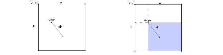
Notice how the starting point (origin) is also a vertex of the sub cell and that the ray is traveling away from it? This is a useful property that we’ll need later on to determine exactly which side the ray is going to intersect.
Each one of these sub cells covers a direction range of 90 degrees. You may also notice from the image below that sometimes the height or width of the sub cell are negative.
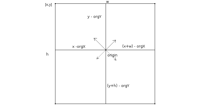
It is necessary to keep the original sign of these values for correct vector scaling that we’ll be doing with
traverse-cell.
(defn sub-cell
  [paren org dir]
  (let [org-x  (nth org 0)
        org-y  (nth org 1)
        width  (if (< (nth dir 0) 0)
                 (- (:x paren) org-x)
                 (- (+ (:x paren) (:w paren)) org-x))
        height (if (< (nth dir 1) 0)
                 (- (:y paren) org-y)
                 (- (+ (:y paren) (:h paren)) org-y))]
    (assoc cell
           :x org-x
           :y org-y
           :w width
           :h height)))
Finding the parent cell
Finding the parent cell of a point by checking if it’s within a certain range might seem like the obvious solution at first, but there’s a catch!
Let’s think about for a moment what do we mean when we say a point is on the grid? The first thing we might imagine is the grid being a border between the cells, something that has a thickness, a kind of “no man’s land”, but in reality all our cells are right next to each other. There is no separating border between them. So when we say that a point is on the grid we actually mean that the point is on the edge of a cell.
The next thing we should think about is how we interpret these points that are on the edges of cells. Suppose we extend a ray to the edge of the current sub cell which would also be the edge of the parent cell. The point we get is the end point of our extension. Now suppose we want to keep extending the ray in the same direction. From which point to we start extending? Do we use the next point in the rays path? If so, how do we know which point comes after the end point? Which point comes after 1? Is it 1.1 or is it maybe 1.01 or even 1.001? It’s clear that we can’t use the point after the end point as our starting point. We obviously have to reuse the end point as the new starting point as if it were a shared point between two cells.
Since we have concluded that the end points can also be a starting points, we can see that the points on the edges of cells are actually in a sort of limbo, where they could potentially belong either an end of one cell or a beginning of another. In the end we do have to decide to which cell does the edge point belong.
The solution to this ambiguity is to take the direction of the ray into account. In other words we can think of the edge point belonging to the cell to which it is facing.
(defn parent-cell
  [org dir]
  (assoc cell
         :x (if (> (nth dir 0) 0)
              ;; The direction is positive meaning the point belongs to the
              ;; current cell so just round to an integer.
              (int (nth org 0))
              ;; The direction is negative which means that the point belongs
              ;; to the previous cell. The call to ceil is to round non grid
              ;; points to integers.
              (.ceil js/Math (- (nth org 0) 1)))
         :y (if (> (nth dir 1) 0)
              (int (nth org 1))
              (.ceil js/Math (- (nth org 1) 1)))
         :w 1
         :h 1))
Traversing the sub cell
Now that we have the parent cell and the sub cell through which the ray is traveling, we need to extend the ray to meet one of the sides of the sub cell. We can do that by scaling the ray’s direction vector to fit the distance between the starting point (origin) of the ray and a side of the cell. But how do we know by how much do we need to scale the vector to fit this length? We need to find a scale factor with which to multiply both components of the direction vector. But before we can do this we first have to figure out to which one of the two possible sides does the vector point to.
To figure this out, we take into account the fact that the origin is also a vertex of the sub cell. Knowing this, we can draw a diagonal from the origin.
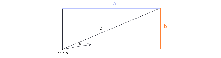
With the diagonal in the picture it’s really easy to tell at which side the vector is pointing at. We simply check where the direction vector is in the relation to the diagonal. You can see that if the direction vector is passing below the diagonal it will have to intersect with b, conversely if it is passing above it it will intersect with a. We can tell where the ray is in relation to the diagonal by comparing the angles of the two.
Before we can compare their angles we have to find them first. To get the direction vector’s angle we simply take the arcsine of the direction vectors Y component since it’s already normalized. To get the angle of the diagonal we first have to scale it to 0-1 range and then take the arcsine.
ray-angle      = |asin(dirY)|
diagonal-angle = |asin(cell-h / √(cell-h² + cell-w²))|
You might notice that we also take the absolute value of both. This is because that if we didn’t, we would have two cases of angle comparisons, one when the direction and the diagonal angles are positive, and one when they are negative. For example when both angles are negative, they are a mirror image of the positive case and thus the angle comparison of the two would also has to be inverted since we’re dealing with negative values. By taking the absolute value of both we reduce the check to only one case.
Depending on which side the direction vector is pointing at, we scale the direction vector to meet that side. There are two possible cases for the scale factor. One is when the ray intersects the side that represents the height of the cell in which case the scale factor would be the sub cell width divided by the direction vector’s X component. This is because we are traversing the width of the sub cell to reach the side that represents the height. The other case is when the ray intersects the side that represents the width. Since we are traversing the height in case, we divide the sub cell’s height with the vector’s Y component. Once we have the scale factor, we multiply the direction vector’s X and Y components to reach the side of a cell.
scale     = (sub-cell-width / dirX) or (sub-cell-height / dirY)
end-point = [dirX * scale, dirY * scale]
(defn traverse-cell
  [quad ray-dir]
  (let [x (nth ray-dir 0)
        y (nth ray-dir 1)
        w (:w quad)
        h (:h quad)
        d (.sqrt js/Math (+ (* w w) (* h h)))
        diagonal-angle (.abs js/Math (.asin js/Math (/ h d)))
        ray-angle      (.abs js/Math (.asin js/Math y))]
    (let [scale (cond
                  (and (<= ray-angle diagonal-angle) (not= x 0)) (/ w x)
                  (and (>  ray-angle diagonal-angle) (not= y 0)) (/ h y)
                  :else 1)]
      [(+ (:x quad) (* x scale))
       (+ (:y quad) (* y scale))])))
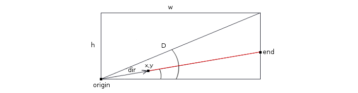
Finding the end point
With these three functions combined we can cast a ray across the grid. To reach the end of the ray we apply
traverse-cell to its output until it returns a point that belongs to a solid cell. Once we have the end point
we can calculate the distance between the original starting point and the end point as shown by this animation:
(defn final-point
  [map org dir]
  (loop [p org]
    (let [par (parent-cell p dir)]
      (if (or (map/point-is-solid map par)
              (and (= (nth dir 0) 0) (= (nth dir 1) 0)))
        [p par]
        (recur
         (traverse-cell (sub-cell par p dir) dir))))))
To wrap it up, we have a cast function that returns a ray and also corrects the ray’s length.
(defn cast
  [map org dir seq ang]
  (let [ep  (final-point map org dir)
        end (nth ep 0)
        par (nth ep 1)
        id  (map/tile-id-at map (:x par) (:y par))
        len (math/point-distance org end)]
    (assoc ray
           :org org
           :end end
           :dir dir
           :len (* len (.cos js/Math (math/to-radians ang)))
           :seq seq
           :tile-id id)))
Casting a fan of rays
In order to render anything interesting we need to cast multiple rays across our field of view. We cast rays in a fan pattern from our eye and cover an angle that represents our field of view. All rays are cast at equal angular distances from each other. In particular rays are cast from -(fov/2) to (fov/2) angles relative to our eye’s forward vector.
We start from -(fov/2) and rotate the direction vector in equal steps. The amount of rotation for each step
depends on the number of rays we are casting.
(defn cast-fan
  [map org fw fov n]
  (let [angle-start (* -1 (/ fov 2))
        angle-step  (/ fov n)
        dir-start   (math/vector-rotate fw angle-start)]
    (loop [step 0 rays []]
      (let [dir (math/vector-rotate dir-start (* step angle-step))
            ang (+ angle-start (* step angle-step))
            ray (cast map org dir step ang)]
        (if (= step n)
          (conj rays ray)
          (recur (inc step) (conj rays ray)))))))
Fish eye effect
If we leave the rays as they are then we’ll get a fish-eye effect which is not what one would expect to see. For example if we looked at a wall, the center of it would bulge out while its sides would curve away from us giving us a fish eye view effect.
Our problem here is that we are casting all rays from a point. In essence this means that all rays are incorrectly projected onto a point instead of a line. This line can be thought of as a camera lens in front of the eye onto which everything is projected. What we need now is a way to correct the ray lengths so that they would appear as if they were cast from a line perpendicular to the direction we are facing instead of our eye point.
These is what the rays look like pre-correction:
You can see that all lengths are of different sizes, but that’s not exactly what we are trying to get. Longer rays on the sides will naturally make the wall curve away from us so we need a way to scale them to a length that they would have if they were cast from a camera line perpendicular to the direction we are looking at.
Cosine correction
A popular way to achieve this is to multiply the ray length with the cosine of the angle between the forward direction and the ray direction. As you will later see this is not a 100% correct solution, but it works well enough for most purposes.
The easiest way to see why this works is to illustrate it:
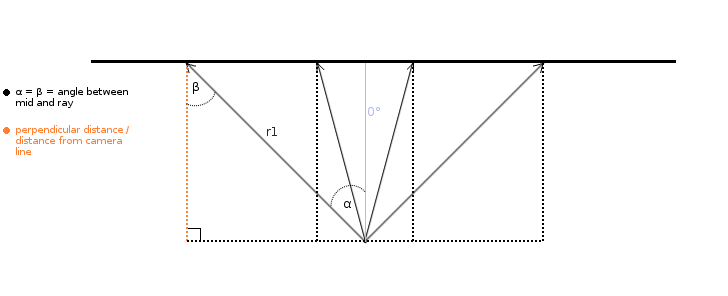
And here’s what we are actually doing achieve this:
-
We can see that angle α = β = the angle between the ray and the forward vector (0°)
-
You can see that in this example the ray (r1), the camera line and the distance from the camera line to the wall (which is the distance we are trying to get) form a right triangle.
-
Notice that the distance from the camera line to the wall (orange dotted line) is actually the cosine of angle β a.k.a. the adjacent side.
-
The original (r1) rays length is actually the hypotenuse of this right triangle.
-
Since we now know the value of angle β, we can get the corrected length by multiplying the hypotenuse (r1) with the
cosof β to scale it to an appropriate size.
Here’s a concrete example to better illustrate this:
-
Angle α = β = 45°
-
Original ray length (hypotenuse) is 10.
-
We call the
cosfunction on angle β and get 0.707 which means that cosine of β (aka the adjacent side of β) is 70.7% of the length of the hypotenuse. -
We multiply the ray (hypotenuse) length with 0.707 to scale it down and get the actual length of the camera line which would in this case be 7.07. We now have the corrected length for that ray.
When we render our columns with this type of correction we get this:
It looks much better, but it still has a flaw. If you look closely you can see that the wall is slightly curved. This is not much of a problem with relatively narrow fields of view, but it becomes much more apparent with wider FOVs. This problem is also hidden when we look straight at the wall. But as soon as we turn the camera we can see the curve.
The actual problem here is that each ray traces an equal angular distance and not an equal surface area of the object it hits. If we remember, we actually use the rays to represent equally spaced columns on the screen. This is where this problem comes from.
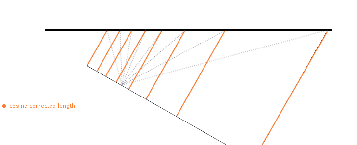
At first glance it might seem that the corrected lengths are following a straight line, but since they all represent an equal portion of the screen or more precisely a column of the screen, we see that they actually form a curve once they are evenly spaced out.
We can see what the curve would look like once we make all rays equally spaced apart:
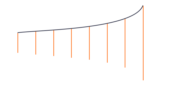
If we were to render this wall it would appear warped. Of course this curve would be flipped since the screen column heights are inversely proportional to ray lengths. You can also imagine that by moving these lines close together, as they would be in more narrow FOVs, that the curve would be less pronounced.
In general if we stick with narrow enough fields of view this solution is good enough. There are of course other ways to cast rays and get better results but approach is probably the simplest.
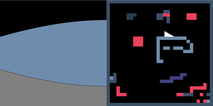
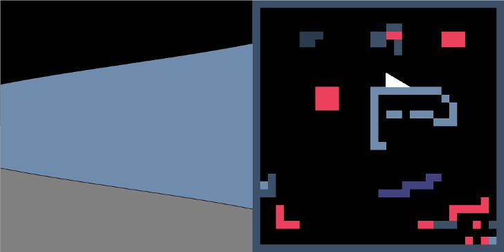
Drawing the scene
Once we have cast all of our the rays we finally have all the information needed for drawing a scene! To draw it we use each ray to represent a column on the screen, where the column height is the screen height divided by the ray length.
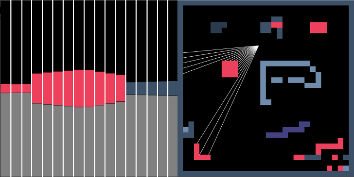
You can see from the image above that the column height is inversely proportional to the ray length. The shorter the ray the close the object and the taller the column we draw and vice versa.
The image also shows a floor which is drawn before the columns by coloring the lower half of the viewport.
(defn draw-columns
  [context viewport rays]
  (do (.save context)
      (let [vp-x    (:x viewport)
            vp-y    (:y viewport)
            vp-h    (:h viewport)
            vp-w    (:w viewport)
            horizon (/ vp-h 2)
            n-rays  (count rays)
            width   (/ vp-w n-rays)]
        (doseq [ray rays]
          (let [n     (:seq ray)
                color (:tile-id ray)
                h     (/ vp-h (:len ray))
                x     (.ceil js/Math (+ vp-x (* n width)))
                y     (/ (- vp-h h) 2)]
            (do (.beginPath context)
                (aset context "fillStyle" (get-color color))
                (.rect context x y width h)
                (.fill context)
                (.closePath context)
    (.restore context)))))))
And so there we have it, a simple and a fully functional raycaster!